A Gentle Introduction to Optimal Power Flow
This post has been originally published here.
In an earlier blog post, we discussed the power flow problem, which serves as the key component of a much more challenging task: the optimal power flow (OPF). OPF is an umbrella term that covers a wide range of constrained optimization problems, the most important ingredients of which are: variables that optimize an objective function, some equality constraints, including the power balance and power flow equations, and inequality constraints, including bounds on the variables. The sets of variables and constraints, as well as the form of the objective, will vary depending on the type of OPF. We first derive the most widely used OPF variant, the economic dispatch problem, which aims to find a minimum cost solution of power demand and supply in the electricity grid. Then, we will briefly review other basic types of OPF. We will see that, unlike the power flow problem, OPF is generally rather expensive to solve. Therefore, we will discuss approximations (known as relaxations) that simplify the original model, as well as computational intelligence and machine learning techniques that try to reduce computational costs.
The power flow problem
In our previous blog post, we introduced the concept of the power flow problem and derived the equations for a simple and for an improved model. Because OPF relies on the power flow problem, we present here the final equations of the improved power flow model. Let $\mathcal{N}$ denote the set of buses (represented by nodes in the corresponding graph of the power grid), and $\mathcal{E}, \mathcal{E}^{R} \subseteq \mathcal{N} \times \mathcal{N}$ the sets of forward and reverse orientations of transmission lines or branches (represented by directed edges in the corresponding graph of the power grid). Further, let $\mathcal{G}_{i}$, $\mathcal{L}_{i}$ and $\mathcal{S}_{i}$ denote the sets of generators, loads and shunt elements that belong to bus $i$. Similarly, the sets of all generators, loads and shunt elements are designated by $\mathcal{G} = \bigcup \limits_{i \in \mathcal{N}} \mathcal{G}_{i}$, $\mathcal{L} = \bigcup \limits_{i \in \mathcal{N}} \mathcal{L}_{i}$ and $\mathcal{S} = \bigcup \limits_{i \in \mathcal{N}} \mathcal{S}_{i}$, respectively. Power flow models explicitly describe the power balance at each bus, based on Tellegen's theorem: \begin{equation} S_{i}^{\mathrm{gen}} - S_{i}^{\mathrm{load}} - S_{i}^{\mathrm{shunt}} = S_{i}^{\mathrm{trans}} \qquad \forall i \in \mathcal{N}. \label{balance} \end{equation} Eq. \eqref{balance} states that the injected power by the connected generators ($S_{i}^{\mathrm{gen}}$) into the bus, reduced by the connected loads ($S_{i}^{\mathrm{load}}$) and shunt elements ($S_{i}^{\mathrm{shunt}}$), is equal to the transmitted power from and to the adjacent buses ($S_{i}^{\mathrm{trans}}$). There are two basic power flow models: the bus injection model (BIM) and the branch flow model (BFM) that are based on the undirected and directed graph representation of the power grid, respectively. In this discussion, we focus on the BFM-based OPF, but we note that an equivalent OPF formulation can be derived from the BIM. Also, we will use the improved power flow model that we described in the previous blog post. Under this model, the BFM has four sets of equations: the first set expresses the power balance for each bus, the second set is the series current of the $\pi$-section model for each transmission line and the last two sets are the (asymmetric) power flows for the two directions of each transmission line: \begin{equation} \begin{aligned} & \sum \limits_{g \in \mathcal{G}_{i}} S_{g}^{G} - \sum \limits_{l \in \mathcal{L}_{i}} S_{l}^{L} - \sum \limits_{s \in \mathcal{S}_{i}} \left( Y_{s}^{S} \right)^{*} \lvert V_{i} \rvert^{2} \\ & \qquad \quad \ = \sum \limits_{(i, j) \in \mathcal{E}} S_{ij} + \sum \limits_{(k, i) \in \mathcal{E}^{R}} S_{ki} \hspace{2.2em} \forall i \in \mathcal{N}, \\ & I_{ij}^{s} = Y_{ij} \left( \frac{V_{i}}{T_{ij}} - V_{j} \right) \hspace{5.1em} \forall (i, j) \in \mathcal{E}, \\ & S_{ij} = V_{i} \left( \frac{I_{ij}^{s}}{T_{ij}^{*}} + Y_{ij}^{C} \frac{V_{i}}{\lvert T_{ij} \rvert^{2}}\right)^{*} \hspace{1.7em} \forall (i, j) \in \mathcal{E}, \\ & S_{ji} = V_{j} \left( -I_{ij}^{s} + Y_{ji}^{C}V_{j} \right)^{*} \hspace{3.8em} \forall (j, i) \in \mathcal{E}^{R}, \\ \end{aligned} \label{bfm_concise} \end{equation} where $S_{g}^{G}$ and $S_{l}^{L}$ represent the complex powers of generator $g$ and load $l$; $Y_{s}^{S}$ is the admittance of shunt element $s$, and $V_{i}$ is the complex voltage of bus $i$. Also, $I_{ij}^{s}$ and $S_{ij}$ denote the series current and power flow; $Y_{ij}$ and $Y_{ij}^{C}$ represent the series admittance and shunt admittance; and $T_{ij}$ designates the complex tap ratio of the $\pi$-section model of branch $i \to j$.
Table 1. Comparison of the improved BIM and BFM formulations of power flow. For each formulation, we show the complex variables (and their real components), the total number of complex (and corresponding real) variables, and the number of complex (and corresponding real) equations. $N = \lvert \mathcal{N} \rvert$, $E = \lvert \mathcal{E} \rvert$, $G = \lvert \mathcal{G} \rvert$ and $L = \lvert \mathcal{L} \rvert$ denote the total number of buses, transmission lines, generators and loads. The variables $v_{i}$, $\delta_{i}$, $i_{ij}^{s}$ and $\gamma_{ij}^{s}$ designate the voltage magnitude and angle of bus $i$, and the magnitude and angle of series current flowing from bus $i$ to bus $j$. The variables $p$ and $q$ denote the active and reactive components of the corresponding complex powers.| Formulation | Variables | Number of variables | Number of equations |
|---|---|---|---|
| BIM | $V_{i} = (v_{i} e^{\mathrm{j}\delta_{i}})$ $S_{g}^{G} = (p_{g}^{G} + \mathrm{j} q_{g}^{G})$ $S_{l}^{L} = (p_{l}^{L} + \mathrm{j} q_{l}^{L})$ |
$N + G + L$ $(2N + 2G + 2L)$ |
$N$ $(2N)$ |
| BFM | $V_{i} = (v_{i} e^{\mathrm{j}\delta_{i}})$ $S_{g}^{G} = (p_{g}^{G} + \mathrm{j} q_{g}^{G})$ $S_{l}^{L} = (p_{l}^{L} + \mathrm{j} q_{l}^{L})$ $I_{ij}^{s} = (i_{ij}^{s} e^{\mathrm{j} \gamma_{ij}^{s}})$ $S_{ij} = (p_{ij} + \mathrm{j} q_{ij})$ $S_{ji} = (p_{ji} + \mathrm{j} q_{ji})$ |
$N + G + L + 3E$ $(2N + 2G + 2L + 6E)$ |
$N + 3E$ $(2N + 6E)$ |
The economic dispatch problem
The first OPF model we discuss is a specific variant of the economic dispatch (ED) model, which tries to find the economically optimal (i.e. lowest possible cost) output of the generators that meets the load and physical constraints of the power system. We first present the elements of an ED formulation using the improved BMF model. (The full optimization problem can be found in the Appendix). Then we discuss the interior-point method, which is one of the most widely used techniques to solve ED problems.
Variables
In power flow problems, the number of equations determines the maximum number of unknown variables for which the non-linear system can be solved. For example, as shown in Table 1, BIM has $N+G+L$ complex variables and $N$ complex equations, which means that $G+L$ variables need to be specified for the problem to be uniquely solvable. In ED, the variables are basically the same as in the power flow problems, but, as an optimization problem, ED has a higher number of unknown variables. For generality, in this discussion we treat all variables in ED formally as unknown. For variables whose value is specified, we can simply define an equality constraint or, more typically, the corresponding lower and upper bounds with the same specific value. This latter formalism (of using lower and upper bounds) makes the model construction more straightforward, and also follows general practice [Coffrin18]. For the following sections, let $X$ denote all variables in ED.
Objective function
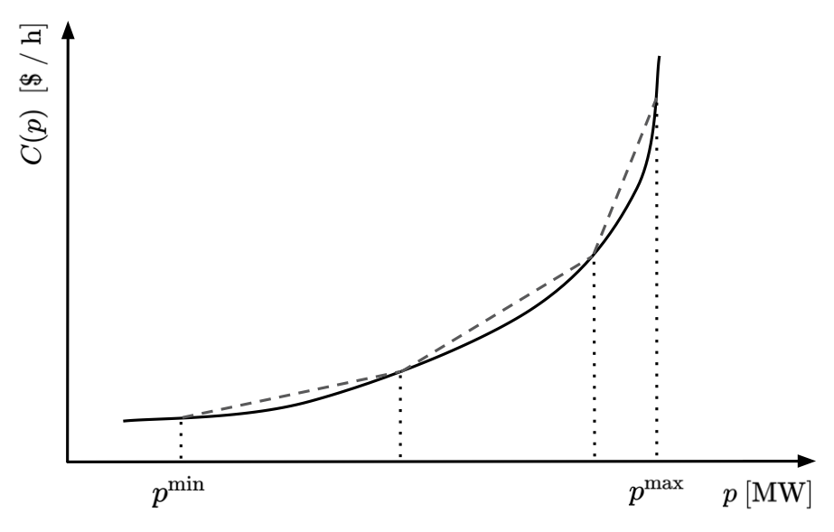
The objective (or cost) function of the most widely used economic dispatch OPF is the cost of the total real power generation. Let $C_{g}(p_{g}^{G})$ denote the individual cost curve of generator $g \in \mathcal{G}$, that is a function solely depending on the (active) power $p_{g}^{G}$ generated by generator $g$. $C_{g}$ is a monotonically increasing function of $p_{g}^{G}$, usually modeled by a quadratic or piecewise linear function. An example of such a function is shown in Figure 1. The objective function $C(X)$ can then be written as: \begin{equation} C(X) = \sum \limits_{g \in \mathcal{G}} C_{g}(p_{g}^{G}). \end{equation} We note that there can be alternative objective functions in OPF that can be used to investigate different features of the power grid [AlRashidi09]. For instance, one can minimize the line loss (i.e. power loss on transmission lines) over the network. Also, the objective function can express additional environmental and economical costs other than pure generation cost. As an example, with the increasing concerns over climate change, multiple studies have suggested that reducing overall emissions from generation should be taken into account in the objective function [Gholami14].
Equality constraints
Equality constraints are expressions of the optimization variables characterized by equations. Equivalently, one can think of an equality constraint as a function of the optimization variables whose function value is fixed. Because power flow equations express fundamental physical laws, they must naturally be contained in any OPF. The power balance equations together with the power flow equations $\eqref{bfm_concise}$ are treated as equality constraints in OPF. In the equations of power flow, the voltage angle differences play a key role, rather than the individual angles. Therefore, without loss of generality we can select a specific value of the voltage angle of a bus as reference and apply an additional equality constraint to this reference bus by setting its voltage angle to zero. We call this the slack or reference bus. In a more general setting, there can be multiple slack buses (i.e. buses used to make up any generation and demand mismatch caused by line losses) and corresponding constraints on their voltage angle. Denoting the set of all reference/slack buses by $\mathcal{R}$ we can write the corresponding constraints for all $r \in \mathcal{R}$ as: $\delta_{r} = 0$.
Inequality constraints
Finally, OPF also includes a set of inequality constraints. Similarly to equality constraints, an inequality constraint can be described by a function of the optimization variables, whose function value is allowed to change within a specified interval. Inequality constraints usually express some physical limitations of the elements of the system. For example, the most typical constraints for the ED problem are:
- lower and upper bounds on voltage magnitude of each bus $i$: $\underline{v}_{i} \le v_{i} \le \overline{v}_{i}$,
- lower and upper bounds on voltage angle difference between all adjacent buses $i$ and $j$: $\underline{\delta}_{ij} \le \delta_{ij} \le \overline{\delta}_{ij}$,
- lower and upper bounds on output active power of each generator $g$: $\underline{p}_{g}^{G} \le p_{g}^{G} \le \overline{p}_{g}^{G}$,
- lower and upper bounds on output reactive power of each generator $g$: $\underline{q}_{g}^{G} \le q_{g}^{G} \le \overline{q}_{g}^{G}$,
- upper bounds on the absolute value of active power flow of all transmission lines: $\lvert p_{ij}\rvert \le \overline{p}_{ij}$,
- upper bounds on the absolute value of reactive power flow of all transmission lines: $\lvert q_{ij}\rvert \le \overline{q}_{ij}$,
- upper bound on the absolute (square) value of complex power flow of all transmission lines: $\lvert S_{ij}\rvert^{2} = p_{ij}^{2} + q_{ij}^{2} \le \overline{S}_{ij}^{2}$.
OPF variants
So far we have been focusing on one specific OPF problem, a variant of the economic dispatch that is one of the most basic types in the realm of OPF. In this section, we briefly discuss other models. In a more general setting, the task of economic dispatch is to optimize some economic utility function for participants, including both loads and generators. For instance, incorporating both power supply and power demand into the objective function leads to the basic concept of the electricity market. At the optimum, the amount of supply and demand power reflects simple market principles subject to the physical constraints of the system: power is primarily bought from generators offering the lowest prices and primarily sold to loads offering the highest prices. In the so-called volt/var control we optimize the combination of power loss, peak demand, and power consumption, with respect to the voltage level and reactive powers. In the above problems, the set of generators is specified and all of these generators are supposed to contribute to the total power generation. However, in real industrial problems, not all generators in the grid need to be active. Generators differ in many ways besides their generation curve: they have different start up and shut down time scales (i.e. how quickly a generator can reach its operating level and how quickly it can stop running), different costs and ramp rates (i.e. the rates at which a generator can increase or decrease its output), different minimum and maximum power generation, etc. All of these quantities need to be taken into account in the planning procedure. Therefore, it is very much desirable to allow specific generators to not run in the optimization model. In order to select the active generators, electricity grid operators solve the unit commitment (UC) problem. The unit commitment economic dispatch (UCED) problem can be considered an extension of the ED problem, where the set of variables is extended with binary variables, each responsible for including or excluding a specific generator in the optimization. The UC problem is, therefore, a mixed-integer non-linear programming problem, which is even harder to solve computationally. Another aspect that needs to be considered is the security of the grid. Power grids are complex systems that include thousands of buses and transmission lines, where failure of any element can happen occasionally and impact the operation of the power grid significantly. Thus, it is very important to account for such contingencies. The corresponding set of problems is called security constrained optimal power flow (SCOPF) and in combination with ED it is called security constrained economic dispatch (SCED). SCOPF provides a solution not only for the ideal unfailing case, but at the same time for some contingency scenarios as well. These problems are much larger scale problems, including a much larger number of variables and constraints, and requiring costly mixed-integer non-linear programming. For example, the widely used $N-1$ contingency problem addresses all scenarios where a single component fails. Finally, we note that a more general (and very large-scale) problem can be formulated by using both UC and SCOPF, leading to the security constrained unit commitment problem (SCUC).
Solving OPF problems
Solving OPF problems by interior-point methods, as described earlier, is widely used as a reliable standard approach. However, solving such problems by interior-point methods is not cheap, as it requires the computation of the Hessian of the Lagrangian $\nabla_{xx} L(x_{n}, s_{n}, y_{n}, z_{n})$ at each iteration step $n$ as in equation $\eqref{primal_dual}$. Because the required computational time has a disadvantageous superlinear scaling with system size, solving large scale problems can be prohibitively difficult. Moreover, the scaling is even worse for mixed-integer OPF problems. There are several approaches that address this issue by either simplifying the original OPF problem, or by computing approximate solutions.
Convex relaxations
The first set of approximations we discuss is called convex relaxations. The main idea of these approaches is to approximate the original non-convex optimization problem with a convex one. Unlike in non-convex problems, in convex problems any local minimum is a global minimum as well (so convex problems, by definition, can only have a single minimum). There are very straightforward algorithms with excellent convergence rates to solve convex optimization problems [Boyd04] [Nocedal06]. To demonstrate convex relaxations, let us consider the economic dispatch problem with the basic BIM formulation. As it can be shown, this problem — with some slight modification — can be reformulated as a quadratically constrained quadratic program (QCQP) using the complex voltages of the buses [Low14]. In this reformulated optimization problem, the objective function and all (inequality) constraints have a quadratic form in the complex voltages: \begin{equation} \begin{aligned} & \min \limits_{V \in \mathbb{C}^{N}} V^{H}CV, \\ & \mathrm{s.t.} \quad V^{H}M_{k}V \le m_{k} \quad k \in \mathcal{K}, \\ \end{aligned} \label{qcqp} \end{equation} where the superscript $H$ denotes conjugate transpose, $M_{k}$s are Hermitian matrices (i.e. $M_{k}^{H} = M_{k}$), and $m_{k}$s are real-valued vectors specifying the corresponding inequality constraints. QCQP is still a non-convex problem that is also an NP-hard problem. Let $W = VV^{H}$ denote a rank–1 positive semidefinite matrix (i.e. rank$(W) = 1$ and $W \succeq 0$). Using the identity of the trace function for any Hermitian matrix: $V^{H}MV = \mathrm{tr}(MVV^{H}) = \mathrm{tr}(MW)$, we can transform the quadratic forms of problem $\eqref{qcqp}$ to expressions that include $W$ instead of $V$: \begin{equation} \begin{aligned} & \min \limits_{W \in \mathbb{S}}\ \mathrm{tr}(CW), \\ & \mathrm{s.t.} \; \; \; \mathrm{tr}(M_{k}W) \le m_{k} \quad k \in \mathcal{K}, \\ & \quad \quad \ W \succeq 0, \\ & \quad \quad \ \mathrm{rank}(W) = 1, \\ \end{aligned} \end{equation} where $\mathbb{S}$ denotes the space of $N \times N$ symmetric matrices. The above problem is convex in $W$, except for the rank-1 equality constraint. Removing this constraint leads to a semidefinite programming problem (SDP), which is called the SDP relaxation of the OPF. SDP introduces a convex superset of the optimization variables. Other choices of convex supersets yield different relaxations, like chordal or second-order cone programming (SOCP), that can be solved even more efficiently than SDP problems. We note that all of these relaxations provide a lower bound to OPF. For some sufficient conditions these relaxations can be even exact [Low14a]. Also, an advantage of convex relaxation approaches over other approximations is that if a relaxed problem is infeasible, then the original problem is also infeasible.
DC-OPF
One of the most widely used approximations is the DC-OPF approach. Its name is pretty misleading, as this method does not assume the use of direct current (as opposed to alternating current), although it removes the reactive power flow equations and the corresponding variables and constraints. The DC approximation is, in fact, a linearization of the original OPF problem (which is sometimes called AC-OPF). In order to demonstrate the simplifications introduced by the DC-OPF approach, we recall that for a simple power flow model the active and reactive powers flowing from bus $i$ to $j$ can be writtes as: \begin{equation} \left\{ \begin{aligned} p_{ij} & = \frac{1}{r_{ij}^{2} + x_{ij}^{2}} \left[ r_{ij} \left( v_{i}^{2} - v_{i} v_{j} \cos(\delta_{ij}) \right) + x_{ij} \left( v_{i} v_{j} \sin(\delta_{ij}) \right) \right], \\ q_{ij} & = \frac{1}{r_{ij}^{2} + x_{ij}^{2}} \left[ x_{ij} \left( v_{i}^{2} - v_{i} v_{j} \cos(\delta_{ij}) \right) + r_{ij} \left( v_{i} v_{j} \sin(\delta_{ij}) \right) \right]. \\ \end{aligned} \right. \label{power_flow_z} \end{equation} DC-OPF makes three major assumptions [Liu09], each of which lead to a simpler expression for the active and reactive power flows ($p_{ij}$ and $q_{ij}$):
- The resistance $r_{ij}$ of each branch is negligible, i.e. $r_{ij} \approx 0$. Applying this assumption to \eqref{power_flow_z}, we obtain: \begin{equation} \left\{ \begin{aligned} p_{ij} & {\ \approx\ } \frac{1}{x_{ij}} \left( v_{i}v_{j}\sin(\delta_{ij}) \right) \\ q_{ij} & {\ \approx\ } \frac{1}{x_{ij}} \left( v_{i}^{2} - v_{i} v_{j} \cos(\delta_{ij}) \right) \end{aligned} \right. \end{equation}
- The bus voltage magnitudes are approximated by one per unit everywhere, i.e. $v_{i} \approx 1$. Using this assumption, we obtain: \begin{equation} \left\{ \begin{aligned} p_{ij} & {\ \approx\ } \frac{\sin(\delta_{ij})}{x_{ij}} \\ q_{ij} & {\ \approx\ } \frac{1 - \cos(\delta_{ij})}{x_{ij}} \end{aligned} \right. \end{equation}
- The voltage angle difference of each branch is very small, i.e. $\cos(\delta_{ij}) \approx 1$ and $\sin(\delta_{ij}) \approx \delta_{ij}$. Applying this assumption leads to our final form: \begin{equation} \left\{ \begin{aligned} p_{ij} & {\ \approx\ } \frac{\delta_{ij}}{x_{ij}}, \\ q_{ij} & {\ \approx\ } 0. \end{aligned} \right. \end{equation}
Computational intelligence and machine learning
The increasing volatility in grid conditions due to the integration of renewable resources (such as wind and solar) creates a desire for OPF problems to be solved in near real-time to have the most accurate state of the system. Satisfying this desire requires grid operators to have the computational capacity to solve consecutive instances of OPF problems, and do so with fast convergence. However, this task is rather challenging for large-scale OPF problems—even when using the DC-OPF approximation. Therefore, as an alternative to interior-point methods, there has been intense research in the computational intelligence [AlRashidi09] and machine learning [Hasan20] communities. Below we provide a list of some well-known approaches. Computational intelligence [AlRashidi09] techniques for solving OPF:
- optimization algorithms that do not require second derivatives, like the L-BFGS-B method, coordinate-descent algorithm, simulated annealing, particle swarm optimization and ant colony optimization;
- evolutionary algorithms like evolutionary programming and evolutionary strategies;
- genetic algorithms;
- fuzzy set theory.
- direct prediction of OPF variables;
- prediction of set-points of OPF variables for subsequent warm-starts of interior-point methods;
- prediction of the active constraints of OPF in order to build and solve significantly smaller reduced OPF problems.
Appendix A: the economic dispatch problem using BFM
Putting everything together, the form of the economic dispatch OPF with BFM is as follows: \begin{equation} \begin{aligned} & \textbf{Variables:} \\ & \quad X^{\mathrm{BFM}} \begin{cases} V_{i} = (v_{i}, \delta_{i}) \hspace{10.4em} \forall i \in \mathcal{N} \\ S_g^{G} = (p_{g}^{G}, q_{g}^{G}) \hspace{9.1em} \forall g \in \mathcal{G} \\ S_{ij} = (p_{ij}, q_{ij}) \hspace{7.8em} \forall (i, j) \in \mathcal{E} \\ S_{ji} = (p_{ji}, q_{ji}) \hspace{7.8em} \forall (j, i) \in \mathcal{E}^{R} \\ I_{ij}^{s} = (i_{ij}^{s}, \gamma_{ij}^{s}) \hspace{8.1em} \forall (i, j) \in \mathcal{E} \\ \end{cases} \\[1em] & \textbf{Objective function:} \\ & \quad \min \limits_{X^{\mathrm{BFM}}} \sum \limits_{g \in \mathcal{G}} C_{g}(p_{g}^{G}) \\[1em] & \textbf{Constraints:} \\ & \quad \mathcal{C}^{\mathrm{PB}} \hspace{0.8em} \begin{cases} \sum \limits_{g \in \mathcal{G}_{i}} S_{g}^{G} - \sum \limits_{l \in \mathcal{L}_{i}} S_{l}^{L} - \sum \limits_{s \in \mathcal{S}_{i}} \left( Y_{s}^{S} \right)^{*} \lvert V_{i} \rvert^{2} \\ \hspace{2.7em} \ = \sum \limits_{(i, j) \in \mathcal{E}} S_{ij} + \sum \limits_{(k, i) \in \mathcal{E}^{R}} S_{ki} \hspace{2.5em} \forall i \in \mathcal{N} \\ \end{cases} \\ & \quad \mathcal{C}^{\mathrm{REF}} \hspace{0.6em} \begin{cases} \delta_{r} = 0 \hspace{13.1em} \forall r \in \mathcal{R} \\ \end{cases} \\ & \quad \mathcal{C}^{\mathrm{BFM}} \hspace{0.2em} \begin{cases} I_{ij}^{s} = Y_{ij} \left( \frac{V_{i}}{T_{ij}} - V_{j} \right) \hspace{5.7em} \forall (i, j) \in \mathcal{E} \\ S_{ij} = V_{i} \left( \frac{I_{ij}^{s}}{T_{ij}^{*}} + Y_{ij}^{C} \frac{V_{i}}{\lvert T_{ij} \rvert^{2}}\right)^{*} \hspace{3.1em} \forall (i, j) \in \mathcal{E} \\ S_{ji} = V_{j} \left( -I_{ij}^{s} + Y_{ji}^{C}V_{j} \right)^{*} \hspace{3.6em} \forall (j, i) \in \mathcal{E}^{R} \\ \end{cases} \\ & \quad \mathcal{C}^{\mathrm{INEQ}} \begin{cases} \underline{v}_{i} \le v_{i} \le \overline{v}_{i} \hspace{10.7em} \forall i \in \mathcal{N} \\ \underline{p}_{g}^{G} \le p_{g}^{G} \le \overline{p}_{g}^{G} \hspace{9.6em} \forall g \in \mathcal{G} \\ \underline{q}_{g}^{G} \le q_{g}^{G} \le \overline{q}_{g}^{G} \hspace{9.6em} \forall g \in \mathcal{G} \\ \underline{\delta}_{ij} \le \delta_{ij} \le \overline{\delta}_{ij} \hspace{8.2em} \forall (i, j) \in \mathcal{E} \\ \lvert p_{ij}\rvert \le \overline{p}_{ij} \hspace{10.1em} \forall (i, j) \in \mathcal{E} \cup \mathcal{E}^{R} \\ \lvert q_{ij}\rvert \le \overline{q}_{ij} \hspace{10.2em} \forall (i, j) \in \mathcal{E} \cup \mathcal{E}^{R} \\ \lvert S_{ij}\rvert^{2} = p_{ij}^{2} + q_{ij}^{2} \le \overline{S}_{ij}^{2} \hspace{4.7em} \forall (i, j) \in \mathcal{E} \cup \mathcal{E}^{R} \\ \end{cases} \\ \end{aligned} \label{opf_bmf} \end{equation} $\mathcal{C}^{\mathrm{PB}}$, $\mathcal{C}^{\mathrm{REF}}$, and $\mathcal{C}^{\mathrm{BFM}}$ denote the equality sets for the power balance, the voltage angle of reference buses, and the improved BFM. $\mathcal{C}^{\mathrm{INEQ}}$ is the set of inequality constraints.
Appendix B: the DC-OPF economic dispatch problem
\begin{equation} \begin{aligned} & \textbf{Variables:} \\ & \quad X^{\mathrm{DC}} \begin{cases} \delta_{i} \hspace{14.0em} \forall i \in \mathcal{N} \\ p_{g}^{G} \hspace{13.5em} \forall g \in \mathcal{G} \\ p_{ij} \hspace{12.0em} \forall (i, j) \in \mathcal{E} \\ \end{cases} \\[1em] & \textbf{Objective function:} \\ & \quad \min \limits_{X^{\mathrm{DC}}} \sum \limits_{g \in \mathcal{G}} C_{g}(p_{g}^{G}) \\[1em] & \textbf{Constraints:} \\ & \quad \mathcal{C}^{\mathrm{PB}} \hspace{0.9em} \begin{cases} \sum \limits_{g \in \mathcal{G}_{i}} p_{g}^{G} - \sum \limits_{l \in \mathcal{L}_{i}} p_{l}^{L} = \sum \limits_{(i, j) \in \mathcal{E}} p_{ij} \hspace{3.0em} \forall i \in \mathcal{N} \\ \end{cases} \\ & \quad \mathcal{C}^{\mathrm{REF}} \hspace{0.5em} \begin{cases} \delta_{r} = 0 \hspace{11.9em} \forall r \in \mathcal{R} \\ \end{cases} \\ & \quad \mathcal{C}^{\mathrm{DC}} \hspace{0.8em} \begin{cases} p_{ij} = \frac{\delta_{ij}}{x_{ij}} \hspace{9.3em} \forall (i, j) \in \mathcal{E} \\ \end{cases} \\ & \quad \mathcal{C}^{\mathrm{INEQ}} \begin{cases} \underline{v}_{i} \le v_{i} \le \overline{v}_{i} \hspace{9.4em} \forall i \in \mathcal{N} \\ \underline{p}_{g}^{G} \le p_{g}^{G} \le \overline{p}_{g}^{G} \hspace{8.3em} \forall g \in \mathcal{G} \\ \underline{\delta}_{ij} \le \delta_{ij} \le \overline{\delta}_{ij} \hspace{6.9em} \forall (i, j) \in \mathcal{E} \\ \lvert p_{ij}\rvert \le \overline{p}_{ij} \hspace{8.8em} \forall (i, j) \in \mathcal{E} \\ \end{cases} \\ \end{aligned} \label{opf_dc} \end{equation} $\mathcal{C}^{\mathrm{PB}}$, $\mathcal{C}^{\mathrm{REF}}$, and $\mathcal{C}^{\mathrm{DC}}$ denote the equality sets for the power balance, the voltage angle of reference buses, and the DC-OPF power flow. $\mathcal{C}^{\mathrm{INEQ}}$ is the set of inequality constraints.
References
[Coffrin18]: C. Coffrin, R. Bent, K. Sundar, Y. Ng and M. Lubin, "PowerModels. JL: An Open-Source Framework for Exploring Power Flow Formulations", Power Systems Computation Conference (PSCC), pp. 1, (2018).
[AlRashidi09]: M. R. AlRashidi and M. E. El-Hawary, "Applications of computational intelligence techniques for solving the revived optimal power flow problem", in Electric Power Systems Research, 79, (2009).
[Gholami14]: A. Gholami, J. Ansari, M. Jamei and A. Kazemi, "Environmental/economic dispatch incorporating renewable energy sources and plug-in vehicles", in IET Generation, Transmission & Distribution, 8, pp. 2183, (2014).
[Nocedal06]: J. Nocedal and S. J. Wright, "Numerical Optimization", New York: Springer, (2006).
[Wachter06]: A. Wächter and L. Biegler, "On the implementation of an interior-point filter line-search algorithm for large-scale nonlinear programming" Math. Program. 106, pp. 25, (2006).
[Boyd04]: S. Boyd and L. Vandenberghe, "Convex Optimization", New York: Cambridge University Press, (2004).
[Low14]: S. H. Low, "Convex Relaxation of Optimal Power Flow—Part I: Formulations and Equivalence", in IEEE Transactions on Control of Network Systems, 1, pp. 15, (2014).
[Low14a]: S. H. Low, "Convex Relaxation of Optimal Power Flow—Part II: Exactness", in IEEE Transactions on Control of Network Systems, 1, pp. 177, (2014).
[Liu09]: H. Liu, L. Tesfatsion and A. A. Chowdhury, "Locational marginal pricing basics for restructured wholesale power markets", IEEE Power & Energy Society General Meeting, pp. 1, (2009).
[Baker19]: K. Baker, "Solutions of DC OPF are Never AC Feasible", arXiv:1912.00319, (2019).
[Hasan20]: F. Hasan, A. Kargarian and A. Mohammadi, "A Survey on Applications of Machine Learning for Optimal Power Flow", IEEE Texas Power and Energy Conference (TPEC), pp. 1, (2020).